Wasserstein Distance, Contraction Mapping, and Modern RL Theory
Classic Math Formulations And Their Impact on Modern RL

Concepts and relations explored by mathematicians with some application in mind — turn out decades later to be the unexpected solutions to problems they initially never imagined. Riemann’s geometry discovered only for pure reason- with absolutely no application in mind, later was used by Einstein to explain space-time fabric and general relativity.
In Reinforcement Learning (RL) an agent seeks an optimal policy for a sequential decision making problem. The common approach to reinforcement learning which models the expectation of this return, or value. But the recent advances in RL which comes under the banner of “Distributional RL” focuses on the distribution of the random return R received by an agent. State-action values can be explicitly treated as a random variable Z whose expectation is the value Q

Normal Bellman operator B (Eq-1) plays a crucial role in approximating the Q values by iteratively minimise the L-square distance between Q and BQ (TD-learning).

Similarly Distributional Bellman operator Ⲧπ approximates the Z values by iteratively minimise the DISTANCE between Z and ⲦπZ.
Z and ⲦπZ are not vectors instead they are distributions, how does one calculate distance between 2 different probability distributions? The answers can be many (KL, DL metrics etc) but we are particularly interested in Wasserstein Distance.
What is Wasserstein Distance
Russian mathematician Leonid Vaseršteĭn, who introduced this concept in 1969. Wasserstein Distance is a measure of the distance between two probability distributions. It is also called Earth Mover’s distance, short for EM distance, because informally it can be interpreted as the minimum energy cost of moving and transforming a pile of dirt in the shape of one probability distribution to the shape of the other distribution.

Wasserstein metric(d𝚙) between cumulative distribution functions F, G is defined as:

Where the infimum is taken over all pairs of random variables (U, V ) with respective cumulative distributions F and G. d𝚙(F,G) is also written as

Example
Let us first look at a simple case: suppose we have two discrete distributions f(x) and g(x), defines as follows:
f(1) = .1, f(2) = .2, f(3) = .4, f(4) = .3
g(1) = .2, g(2) = .1, g(3) = .2, g(4) = .5
Let compute the Wasserstein metric (d𝚙) as defined in Eq3:
δ0 = 0.1–0.2 = -0.1
δ1= 0.2–0.1 = 0.1
δ2= 0.4–0.2 = 0.2
δ3= 0.3–0.5 = -0.2
Thus Wasserstein metric (d𝚙) =∑|δi|=0.6
Why Wasserstein Distance
Unlike the Kullback-Leibler divergence, the Wasserstein metric is a true probability metric and considers both the probability of and the distance between various outcome events. Unlike other distance metrics like KL-divergence, Wasserstein distance provide a meaningful and smooth representation of the distance between distributions.
These properties make the Wasserstein well-suited to domains where an underlying similarity in outcome is more important than exactly matching likelihoods.

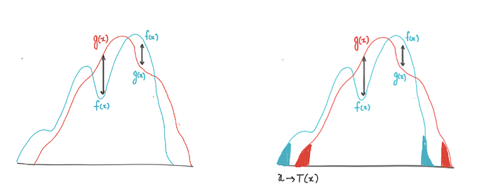
Right plot: The measures between red and blue distributions are the same for KL divergence whereas Wasserstein distance measures the work required to transport the probability mass from the red state to the blue state.
Left plot: Wasserstein distance does have problem. The distance remains same as long as transfer the probability mass remains same regardless of what direction the transfer is happening. Thus, we do not have a way to do inference for the distance.
ɣ-contraction
Contraction mapping plays pivotal mathematical role in the classical analysis of reinforcement learning. Lets first define contraction
Contraction Mapping
A function (or operator or mapping) defined on the elements of the metric space (X, d) is a contraction, if there exists some constant ɣ such that for any two elements of the metric space 𝓧₁ and 𝓧₂, the following condition holds:

This means that after applying the mapping f(.) on the elements 𝓧₁ and 𝓧₂, they got closer to each other by at least a factor ɣ .
Contraction in RL
It is very important to prove contraction as it justifies the usage of distance metric itself. Distribution operator Ⲧπ is used to estimate the Z(x,a) and proving Ⲧπ is a contraction in d𝚙 implies that all moments also converge exponentially quickly.

What contraction tells is that applying operator Ⲧ to 2 different distributions shrinks the distance between them, so choice of distance metric is very important. Now lets try to prove “Distribution Operator Ⲧπ” is contraction in Wasserstein distance(d𝚙).
Proof
3 important properties of Wasserstein metric which helps us prove contraction.


Conclusion
In this blog, we defined Wasserstein distance, discussed its advantages and disadvantages. We justified its usage as a distance metric in distributional- Bellman operator by proving its contraction. But it's just the end of the beginning, Wasserstein distance posses challenge when computing stochastic gradients which renders it ineffective when functional approximations are used. In my next blog, I will discuss how to approximate Wasserstein metric using quantile regression.
Thanks :)
