NLP Zero to One: Recurrent Neural Networks Basics Part(8/30)
Back-Propagation Through Time, Vanishing Gradients, Clipping

Introduction
So far we looked at methods where the long-term dependencies and the contextual order between words is not considered. Even while developing the word embeddings, the order of words is still not considered amongst the context words. The sequence of words play very important role in many NLP tasks. For example “Man bites dog” and “dog bites man” both sentences have same words but the meaning is entirely different. So, our understanding of bag of words so far must extent to word sequences. In this blog, we introduce recurrent neural networks (RNNs) that extend deep learning to sequences and also we will describe the training process for RNN.
Recurrence…
RNN is simple feed-forward network like the neural networks we introduced earlier, it takes a sequence of vectors as input. But there is an extra components with enables it to learn the sequences. This component is called memory/history. Lets try to understand the concept of memory.
As mentioned RNN consumes a sequence of vectors as input and let’s define a the input sequence as X with time steps T, where X = {x1,x2, . . . ,xT } where such that xt is vector input at time t. We then define our memory or history up to time t as ht.
In order to incorporate sequential context into the next time step’s prediction, memory (ht) of the previous time steps in the sequence must be preserved.

The function f(.) maps memory and input to an output at time t. The memory from the previous time step is ht−1, and the input is xt. It very obvious that the output is directly dependent on the result from previous step, this is where the notion of recurrence comes from.
Neural Network..
If the mapping function f(.) is approximated using a neural network, then we call this kind of modelling as recurrent neural network

where W and U are weight matrices which are learnable.


Training of RNN are very similar to feedforward networks which is introduced in previous blog in this series. The usual steps involves calculating the error for a prediction, computing the gradients for each set of weights via back-propagation, and updating the weights according to the gradient descent optimisation method. Though RNN’s training process looks very similar to the feed-forward networks, there is a deviation in the process of computation of gradients. The weight matrix V to the recurrent connection. Therefore, computing the gradient is the exactly same as a standard multi layer perceptron feed forward network.
Back-Propagation Through Time (BPTT)
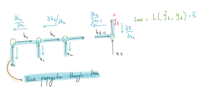
In RNN the weights at all earlier times steps contribute to the output of network, so the weights at all time steps must be computed with gradient descent optimisation method. The gradients are computed by evaluating every path that contributed to the prediction. This process is called back-propagation through time (BPTT).
In the above figure we illustrated how the weights are updated for a loss (Et) that is calculated at time step t. The error for all time steps is the summation of Et ’s and we can sum the gradients for each of the weights in our network (U, V, and W) and update then with the accumulated gradients.
Vanishing Gradients
In multi layer perceptron which is a standard feed forward network, when training neural networks with many layers with back-propagation, the issue of vanishing arises. If you closely observe the gradient in backpropagation, we are multiplying the gradient by the output of each successive layer. This means that the gradients of weights/biases that are present in the layers close to input can be smaller and smaller if the partial derivative terms it picks-up along its way less than 1.
This phenomenon is called vanishing gradients: the gradients can be so small the error that back-propagated to that weight/bias terms in the layer is ineffective in updating any weights. This prevents learning in early layers. The deeper a neural network becomes, the greater a problem this becomes.
Vanishing Gradients in RNN
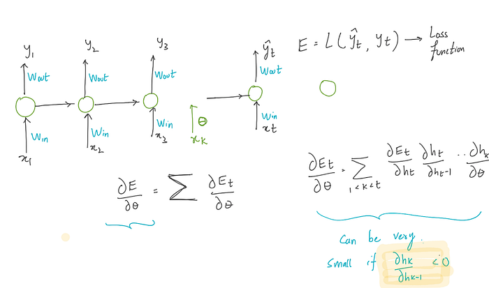
The problem of vanishing gradients is very obvious in RNN. Because of the recurrence aspect, during back-propagation through time, the gradients are multiplied by the weight’s contribution to the error at each time step. The impact of this multiplication at each time step dramatically reduces gradient propagated to the previous time step which will in turn be multiplied again. This causes the same issues as discussed above. when the gradient is very small, the weight update can be negligible and the network doesn’t learn anymore. We can add gates to RNN to combat vanishing gradients.
Note:
Gradient Clipping: It’s a simple way to limit gradient explosion is to force the gradients to a specific range. This prevents the overflow errors when training. Also gradient clipping helps in improving convergence.

Next: NLP Zero to One: LSTM Part(9/40)
Previous: NLP Zero to One: Training Embeddings using Gensim and Visualisation (Part 7/30)

